Overview of Automatic Time Series Forecasting

Online forecasting of a large set of different time series is often required. For instance, a business may want to forecast the sales for all of its products. For such problems the form of each time series can vary significantly meaning that different modelling techniques can be required across the set. However, manually selecting an appropriate model for each time series can be too labour intensive, especially in the case of online learning when this task has to be continually repeated over time. To solve this problem, algorithms can be used to perform model selection automatically.

How automated model selection works

Automated model selection works using the following three steps:

1. Use Time-Series Cross-Validation to generate historical error data of different modelling techniques.
2. Train a model selection algorithm on historical error data.
3. Forecast with the trained model selection algorithm.

These steps can be applied to applied automatically without the need for manual intervention.

1. Time Series Cross-Validation to generate historical error data

Time series cross-validation generates multiple overlapping forecasts prior to the period we are interested in forecasting. For instance, say we are at the time point indicated in Figure 1.2 and want to perform model selection on the three different available models.

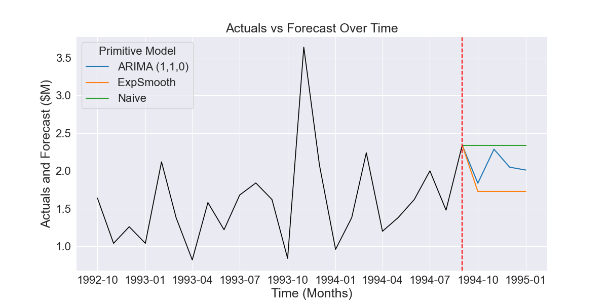
In this case, time series cross-validation would involve collecting the historical forecasts for the prior 12 months, as shown in the Figure 1.2.

The error of these forecasts can then be compared as a basis for model selection.

2. Train a Model Selection Algorithm on historical error data

2.1 Algorithm framework

Model selection algorithms use the error of forecasts generated using cross-validation to decide which model or models should be used in the final forecast.

Model selection algorithms can be described as functions of the loss matrix $\boldsymbol L$ that calculate weights vector $\boldsymbol \beta$ where $\boldsymbol L$ is defined as the error of all $j$ models over $T$ historical periods i.e.

$$ \boldsymbol L = \begin{bmatrix}\ \large{l} _{1,1} & \large{l} _{1,2} & \large{l} _{1,3} & \cdots & \large{l} _{1,J} \\ \large{l} _{2,1} & \large{l} _{2,2} & \large{l} _{2,3} & \cdots & \large{l} _{2,J} \\ \vdots & \vdots & \vdots & \ddots & \vdots \\ \large{l} _{T,1} & \large{l} _{T,2} & \large{l} _{T,3} & \cdots & \large{l} _{T,J} \end{bmatrix} $$

… and where $\boldsymbol \beta$ is defined as the learned weights of all $j$ models i.e.

$$ \boldsymbol \beta = \begin{bmatrix}\beta_{1} \\ \beta_{2} \\ … \\ \beta_{m}\end{bmatrix} \ \ \ \ \ \ \ \ \ \ \
w.r.t\ \ \sum_{j=1}^m\beta_j=1 $$

2.2 FollowTheLeader

The simplest model selection algorithm, called FollowTheLeader, works by picking a single model that has the best historical performance i.e. it selects $j∗$ with the lowest error over all $T$ forecast periods:

$$j* = \underset{j}{\operatorname{argmin}} \sum_{i=1}^{T}\large{l} _{i,j}$$

After finding $j*$, the model weight vector $\boldsymbol \beta$ is calculated as:

$$\boldsymbol \beta = \begin{bmatrix}\ \unicode{x1D7D9} [1= j * ] \\ \unicode{x1D7D9}[2=j*] \\ … \\ \unicode{x1D7D9}[m=j * ]\end{bmatrix}$$

This results in FollowTheLeader assigning the best performing model weight 1 and all other models weight 0.

2.3 AdaptiveHedge

AdaptiveHedge calculates the weights vector $\boldsymbol \beta$ with the following function.

$$ \beta_j = \cfrac{\operatorname{\exp}\bigg(-\epsilon\cdot{\displaystyle\sum\limits_{i=1}^{T} \ (1-\alpha)^{i} \ \large{l}_ {\ T-i,\ j}\bigg)}} {\displaystyle\sum\limits_{j=1}^{M} \operatorname{\exp}\bigg(-\epsilon\cdot{\sum\limits_{i=1}^{T} \ (1-\alpha)^{i}
\large{l}_{\ T-i,\ j} \bigg)}} $$

The algorithm has two main components. Firstly, rather than taking a mean of the loss over the whole period, a weighted average is taken with the weights exponentially decaying as the loss goes back in time away from time point T. This is achieved through the following term:

$$ \large ema({l}_ {j}) = \sum\limits_{i=1}^{T}(1-\alpha)^{i} \ \large{l}_ {\ T-i,\ j}$$

This is the same exponential moving average method used by an exponential smoothing forecasting model.

The algorithms second component is a softmax function that is is applied to exponential moving average component for each model. i.e.  

$$ \large S(\large ema({l}_ {j}),\ \epsilon) = \frac{\operatorname{\exp}\bigg(-\epsilon\cdot \large ema({l}_ {j})\bigg) }{\displaystyle\sum_{j=1}^{M}\operatorname{\exp}\bigg(-\epsilon\cdot \large ema({l}_ {j})\bigg) } $$

This results in AdaptiveHedge producing relatively even weights, with only a slightly higher weight given to a model with a lower error. The differences between the weights can be adjusted using the $ \large \epsilon $ hyperparameter, referred to as the learning rate.

2.4 FollowTheLeader vs AdaptiveHedge intuitive comparison

To gain intuition on how AdaptiveHedge and FollowTheLeader behave we can plot the weights output as the error of three theoretical models changes over time.

Like it’s name suggests, we can see that AdaptiveHedge takes a more moderate hedged approach restricting the difference in model weights to a range with a maximum of 0.5 and a minimum of 0.25. FollowTheLeader, on the other hand, sets weights to the relatively extreme values of 1 or 0 and does so even when the model assigned a weight of 1 is only marginally better than the next best model.

3. Forecast with the trained model selection algorithm

The two steps above have shown how time-series cross-validation data is collected and used to train model selection algorithms. The final step is to use these trained algorithms to make a forecast $\widehat{y}{'}$.

To do so for a time series at time point ${T+h}$ we use the equation:

$$\widehat{y}{'}_{T+h} = \boldsymbol \beta^T \widehat {\boldsymbol Y} _{T+h}$$

Where $\boldsymbol \beta$ is the vector of learnt weights and $\widehat {\boldsymbol Y} _{T+h}$ is the vector of forecasts of the individual models at time point $T+h$ i.e.

$$\widehat {\boldsymbol Y} _ {T+h} = \begin{bmatrix}\ \widehat{y}{} _ {1,T+h} \\ \widehat{y}{} _ {2,T+h} \\ … \\ \widehat{y}{} _ {m,T+h}\end{bmatrix}$$

That is, we use the weights learnt by the models selection algorithm to take a weighted average of the primary forecasts for a given time point.

In the example gone through in section 1. the predictions at each point in the forecasted period show in Fig 1.1. are represented by a $\widehat {\boldsymbol Y} _{T+h}$  vector.

The $\widehat{y}{'}$ forecasts produced by FollowTheLeader and AdaptiveHedge trained on the 12 time series cross-validation forecasts shown in Fig 1.2 produces the forecasts shown bellow in Fig 1.3.

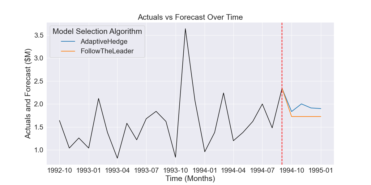
As we can see, FollowTheLeader has picked the best performing exponential smoothing model, while AdaptiveHedge has taken an average of all three with a heavier weighting given to Exponential Smoothing, followed by the ARIMA model.

Conclusion to part 1) How automated model selection works

We’ve now gone through how automated model selection works through an initial stage of time series cross-validation, model selection algorithm training on the forecasts collected and, finally, forecasting with the trained algorithms.

In part 2) we will compare the performance of AdaptiveHedge and FollowTheLeader on the M3 forecasting competition benchmark dataset to show the advantage the AdaptiveHedge can give over FollowTheLeader.